4 min to read
Ray Tracing - Fog
Cover: Ray Tracing in Homogeneous Media, 1024-spp
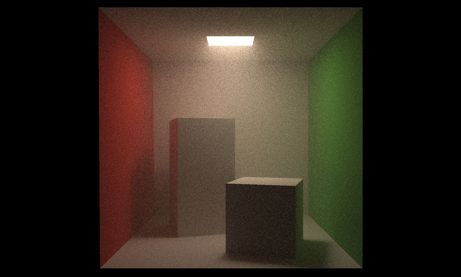
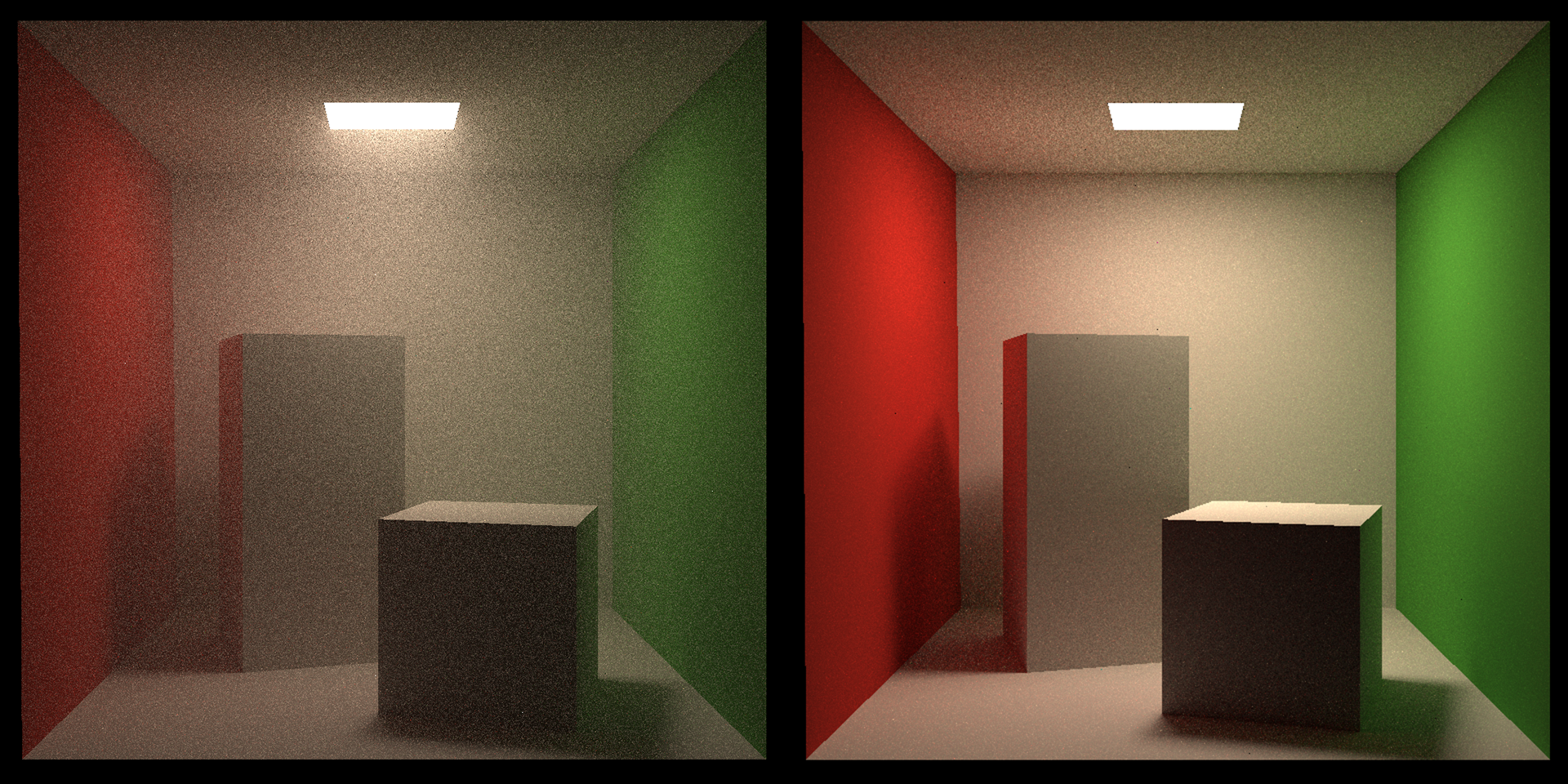 w/wo fog, note the scattering around the light source
Volume Rendering Equation
Since the emission term is easier to calculate than scattering, we only consider scattering and absorption terms here.
Consider a light, its radiance is described by: \(\frac{\partial L(\boldsymbol{x}, \boldsymbol{\omega})}{\partial s} = \mu_s(\boldsymbol{x})\int_{\Omega}f(\boldsymbol{x}, \boldsymbol{\omega'}, \boldsymbol{\omega})L(\boldsymbol{x},\boldsymbol{\omega'})d\boldsymbol{\omega'} - \mu_a(\boldsymbol{x})L(\boldsymbol{x}, \boldsymbol{\omega})\)
Meaning
Scattering
On the right hand side of the formula, the first term represents scattering, where \(\mu_s\) is the scattering coefficient. We consider the incident ray from \(\boldsymbol{\omega'}\), its ratio of contribution in the differential solid angle \(\boldsymbol{\omega'}\) on direction \(\boldsymbol{\omega}\) being \(f(\boldsymbol{x}, \boldsymbol{\omega'}, \boldsymbol{\omega})L(\boldsymbol{x},\boldsymbol{\omega'})\). For isotropic scattering, \(f(\boldsymbol{x}, \boldsymbol{\omega'}, \boldsymbol{\omega})\) becomes \(1/4\pi\).
Absorption
The second term represents absorption. \(\mu_a\) is the absorption coefficient, representing the ratio of photons being absorbed.
Homogeneous and isotropic solution
Solving the equation (with boundary conditions) gives us \(L(\boldsymbol{x}, \boldsymbol{\omega}) = \int_{0}^{z}T(\boldsymbol{x}, \boldsymbol{y})[\mu_a(\boldsymbol{y})L_e(\boldsymbol{y},\boldsymbol{\omega}) + \mu_s(\boldsymbol{y})L_s(\boldsymbol{y}, \boldsymbol{\omega})]d\boldsymbol{y} + T(\boldsymbol{x}, \boldsymbol{z})L_o(\boldsymbol{z}, \boldsymbol{\omega})\), where \(T(\boldsymbol{x}, \boldsymbol{y}) = e^{-\int_{0}^{s}\mu_t(s)ds}\). If we only consider homogeneous (i.e., \(\mu\equiv C\)) and isotropic (i.e., scattering distributes evenly within \(4\pi\) solid angle) media, then the equation can be simplified to \(L(\boldsymbol{x}, \boldsymbol{\omega}) = \int_{0}^{z}e^{-\mu_t s_y}\mu_s\int_{4\pi}f_p(\boldsymbol{\omega}, \boldsymbol{\bar{\omega}})L(\boldsymbol{y}, \boldsymbol{\bar{\omega}})d\boldsymbol{\bar{\omega}}d\boldsymbol{y} + e^{-\mu_t s_z}L_o(\boldsymbol{z}, \boldsymbol{\omega})\).
Monte Carlo Sampling
The sampling of this equation is more challenging than ray casting without media in mainly the following ways:
- Traditional ray casting samples on only the surface, while here we basically need to sample any point in the space;
- We need to sample a double integral. While the idea is similar, it introduces much more noice, thus requiring more time to converge;
- The traditional ray casting will always sample from a light source. It greatly increases hit rate of rays with a few bounds, so we want to keep it. However, we need to make it compatible with sampling within the media.
Sampling the distance
Instead of sampling points in the space and on the surface simultaneously, we sample a distance to estimate how far the ray will travel, and sample a point accordingly. In the homogeneous media where \(\mu_a + \mu_s = \mu_t\), the proportion of light that remains after distance \(t\) is \(e^{-\mu_t t}\). This is also the probability that a photon will survive after such a distance, i.e., \(P(x>t) = e^{-\mu_t t}\).
Using inverse transform sampling, we can sample the distance r.v. \(X\) from a uniform r.v. \(\xi\) by \(x = -\frac{ln(1-\xi)}{\mu_t}\). This can be easily verified by calculating the cdf: \(P(x \le t) = P(\xi < 1 - e^{-\mu_t t}) = 1 - e^{-\mu_t t}\). Now, we know that the photon we are tracing travels distance \(t\) before absorbed/scattered (a fancy term for this is free path). Then we compare \(t\) with the distance \(z\) to the closest surface that the photon could have hit. If \(t < z\), we sample the scattering term. Otherwise, we sample on the surface, which is similar to the traditional ray casting.
Implementation
After some (annoying) calculation and elegant simplification, we can get a rather simple sampling process.
    Vector3f castRay(Ray& ray) {
        float sampleDis = -log(get_random_float()) / miut;
        float intersectDis = intersect_to_ray_origin_distance;
        if (sampleDis < intersectDis) {
            sample the nextRay evenly within 4pi
            return scat / miut * castSpaceRay(nextRay);
        } else {
            if (intersect is light source) return light_source_emission;
            return rayCasting(ray); // rayCasting on surface
        }
    }
This is amazingly simple, e.g., we don’t have any extra coefficient for the surface sampling part (because they cancel out each other)!
To understand the underlying process, I would strongly recommend you read CMU’s rendering lecture, which includes a detailed implementation, and The Siggraph course , especially the distance sampling part, which includes a vivid explanation. Here, I only provide an informal proof of correctness:
\(\langle L \rangle = \frac{\mu_s}{\mu_t}P(X < z)L_s + P(X \ge z)L_o\) \(= \frac{T(t)}{p(t)}\mu_s P(X < z)f(\omega, \bar{\omega})L_s/p(\bar{\omega}) + P(X \ge z)\frac{T(z)}{P(X \ge z)}L_o\), since \(\frac{T(t)}{p(t)} = \frac{1}{\mu_t}\), \(f(\omega, \bar{\omega}) = p(\bar{\omega})\) in isotropic situation, and \(T(z) = P(X \ge z)\).
Therefore, \(\overline{E}(L) = \int_{0}^{z}T(y)\mu_s L_sdy + T(z)L_o\), as desired.
Understanding and parameter choosing
What not mentioned in most essays is how to choose good \(\mu_t\) and \(\mu_s\). Generally, this is related to the size of your scene. To explain this, let’s understand the above implementation in an intuitive way:
- The lighting term is sampled only when sampleDis > intersectDis. This is as if the global illumination is cut down by \(P(X>z)\).
- Part of the energy from the global illumination is scattered, as the other is absorbed.
Empirically, I would set \(\mu_t / \mu_a\) to a very large number, e.g., \(10:1\) to \(50:1\), such that the whole scene is not too dark while the scattering is clearly visible. Regarding their absolute value, I prefer to make the median free path be around half of the depth of the scene to achieve a reasonable proportion between the scattering term and the surface term. A very high \(\mu_t\) would make most of the scene pure black, since the photon can hardly reach a light source. On the other hand, a low \(\mu_t\) would make the media less obvious.